Dart Physics

We have a dart board at the office and have a good time lofting darts in nice, looping arcs. A recent project pushed me back into physics and led me to consider just how sensitive the dart-throwing motion is to small imperfections in angle; how precise do we need to be? Calculating those angular perturbations ($dy/d\theta$ in the coordinates I’ll set up next) requires the kinematics of the problem and provides an opportunity to solve the equations numerically with R.

Setup

Our office dart board is fixed at a location $\mathbf{r}_d = \langle x_d, y_d \rangle = \langle L, 0\rangle$, and a thrower (darter? player?) stands with their throwing elbow at a location $\mathbf{r}_t = \langle 0, -r \rangle$. Here $r$ is the player’s forearm length and things are arranged so a “perfect” 90$^\circ$ release starts from a height $y=0$. Recall that the kinematics derive from Newton’s second law. Assuming a constant gravitational acceleration $g$ near the earth’s surface, we want to solve the equations $$x(t) = x_0 + v_0^{(x)}t, \\ y(t) = y_0 + v_0^{(y)}t - \frac{1}{2}gt^2 .$$ Because there are no forces acting left to right (except for the neglected air drag), the $x$ equation has no acceleration term.

With the above equations come initial conditions: $x_0 = r\cos\theta$ and $y_0 = r(\sin\theta - 1)$ with $\theta$ the release angle – the angle of the player’s forearm at the moment of the throw. The angle $\theta$ is measured conventionally (and unintuitively here) from the forward direction, so a throw vertically upwards would have $\theta = 180^\circ$. Computing $\mathbf{v}_0$ is a little trickier but possible with a bit of trigonometry and calculus; the magnitude is just $v = r d\theta/dt \equiv r\omega$, and one can show that $$v_0^{(x)} = \phantom{-}r\omega\sin\theta,\\ v_0^{(y)} = -r\omega\cos\theta .$$

Solution

To find a solution wherein we hit the bullseye, we fix $x(t_f) = L$ and $y(t_f) = 0$, with $t_f$ the time to target. These definitions specify the solution after some tedious algebra. First, the $x$ equation yields time as a simple function of release angle $\theta$ and angular velocity $\omega$ (or linear velocity $\nu = r\omega$): $$t_f = \frac{L - r\cos\theta}{r\omega\sin\theta} .$$ Intuitively, the time of flight is the ratio of the distance traveled in the $x$ direction to $v_0^{(x)}$. The $t_f$ equation generates a more complicated expression for the angular velocity: $$\omega = \left\{ \frac{g (L - r\cos\theta)^2} {2 r^2\sin\theta \left[ r(1-\sin\theta) - L\cos\theta \right]} \right\}^{1/2} .$$ This one’s harder to interpret, but it has the correct units (s$^{-1}$) and exhibits interesting divergences: $\omega \to \pm\infty$ as $\theta \to 0$, $\pi/2$, $\pi$, etc. Note, too, that the $\pi/2$ divergence differs from its $\pi$ counterpart in that different parts of the denominator go to zero ($\sin\theta$ vs. the term in square brackets).

With the solution in hand we can also find the maximum height of the dart during its flight. The path is a function of $\theta$ and $\omega$, and the maximum height is an extremum of $y(t)$: $0 = \frac{dy}{dt} = v_0^{(y)}-gt$. A check of the second derivative confirms this is, in fact, a maximum, and $$y_\mathrm{max} = r(\sin\theta - 1) + \frac{(L - r\cos\theta)^2}{4\tan^2\theta\left[ r(1-\sin\theta) - L\cos\theta \right]}.$$ The maximum depends on the starting height and also varies with the $x$ distance to be crossed by the dart.

Finally, we can work out an answer to my original question: how sensitive is the solution $y(t)$ to perturbations in angle, $\delta\theta$? The answer comes from the accurate solution $\langle x(t_f) = L, y(t_f) = 0 \rangle$ by computing the derivative $dy/d\theta$ at fixed $\omega$ – the angular frequency of the accurate solution. The derivative is $$\frac{dy}{d\theta}\Bigg\rvert_\omega = (r\cos\theta - L) \left\{ - \frac{1}{\sin^2\theta} + \frac{g}{r^2 \omega^2 \sin\theta} \left[ r + \frac{(r\cos\theta - L)}{\sin\theta \tan\theta} \right] \right\},$$ and this quantity can be interpreted as the vertical distance by which the dart would miss for a small (e.g., $\lesssim 1$ degree) imperfection in the release angle. We could go on to ask similar questions about imperfections in velocity.

Calculation

Now that we have the general solutions, let’s take a look at the results numerically. Start by making a few assignments:

G_EARTH <- 9.8

L <- 10*12 * 2.54/100  # 10 feet
r <- 14    * 2.54/100  # 14 inch forearm
C <- 6*12  * 2.54/100  # 6 more feet

The constant $C$ measures the ceiling height relative to the bullseye, $r$ is the forearm length, and $L$ is the horizontal distance between the player and the board. Here I’ve estimated $L = 10$ feet, $r = 14$ inches, and $C = 6$ feet of clearance. The gravitational constant is, as always, 9.8 meters per squared second. With the constants fixed, I’ve implemented the kinematic equations as functions in R and computed them on a $10^{-4}$ radian grid spanning $\theta \in [0, \pi]$:²

calc <- tibble(
  theta     = seq(pi, 0, -pi*1e-4),
  theta_deg = theta * 180/pi,
  omega     = omega(L = L, r = r, theta = theta),
  vel       = r*omega,
  vel_mph   = vel * 3600 * 100 / 2.54 / 12 / 5280,
  time      = tt(L = L, r = r, theta = theta),
  y0        = r*(sin(theta - 1)),
  ymax      = ymax(L = L, r = r, theta = theta),
  yratio    = ymax/y0,
  ymax_ft   = ymax * 100 / 2.54 / 12,
  hit_ceil  = ymax >= C,
  dy_dtheta = dydtheta(L = L, r = r, theta = theta)
)

The results can be simply divided into two main categories: “standard” vs. “extreme” solutions.

Standard Solutions

I’ve defined standard solutions as those for which (i) the dart doesn’t hit the ceiling and (ii) $\theta \ge 100^\circ$ to separate out the slightly crazier results.

We find, intuitively, that the throw velocity must increase as the release angle approaches 90 degrees. The maximum height and air travel time always decrease as the trajectory flattens, but interestingly the required throw velocity has a minimum value. (In the figures I’m plotting vs. $\varphi = 180^\circ - \theta$; $0^\circ$ corresponds to a vertical upwards throw and $180^\circ$ to a vertical downwards throw.)

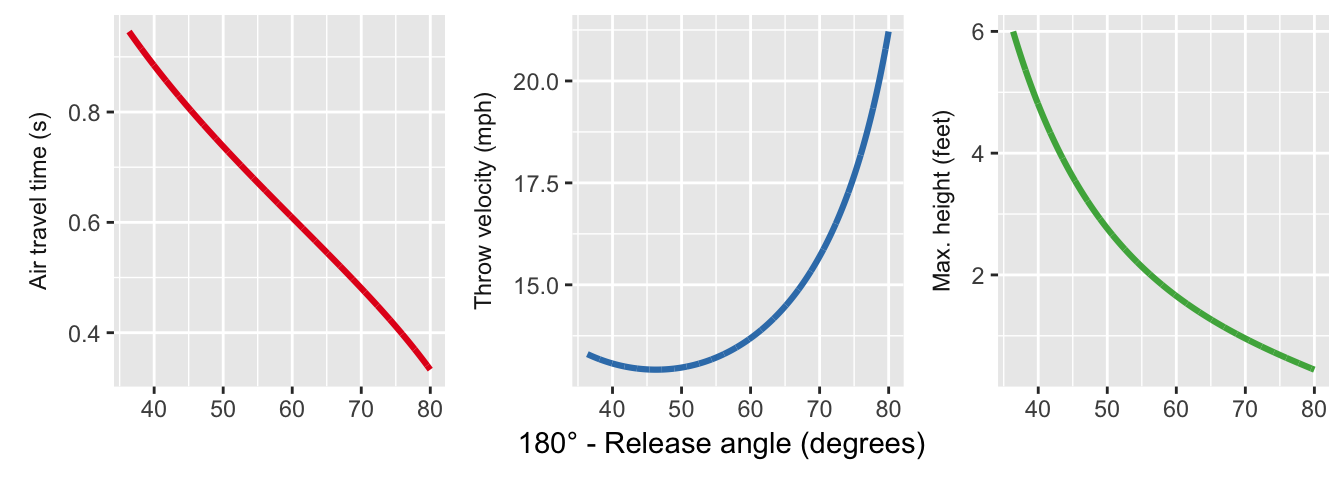
For $\varphi < \varphi_\mathrm{min}$ we have to throw the dart harder because much of its velocity is “wasted” traveling vertically. On the other hand, for $\varphi > \varphi_\mathrm{min}$ we need more velocity to make it to the target before gravity can pull the dart too far. We could take a derivative to find $\varphi_\mathrm{min}$, but since we’re already here we can just find the minimum numerically:

opt_value <- optimize(function(.x) omega(L, r, .x)^2, c(pi/2, pi))
180 - opt_value$minimum * 180/pi

## [1] 46.30904

The minimum is not $45^\circ$, but slightly larger (a flatter trajectory).

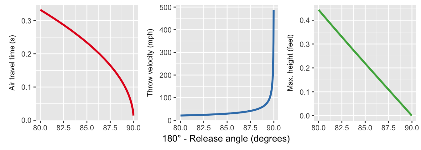
Crazier Solutions

The first set of results not yet considered covers solutions approaching a perfectly horizontal throw. The travel time and maximum height again decrease (the maximum height decreases roughly linearly), but the throw velocity diverges: as $\varphi \to 90^\circ$ the dart needs $v \to \infty$ to hit the bullseye before gravity pulls it off line.

Finally, there’s a slice of the solution for which we need a more vertical headroom:

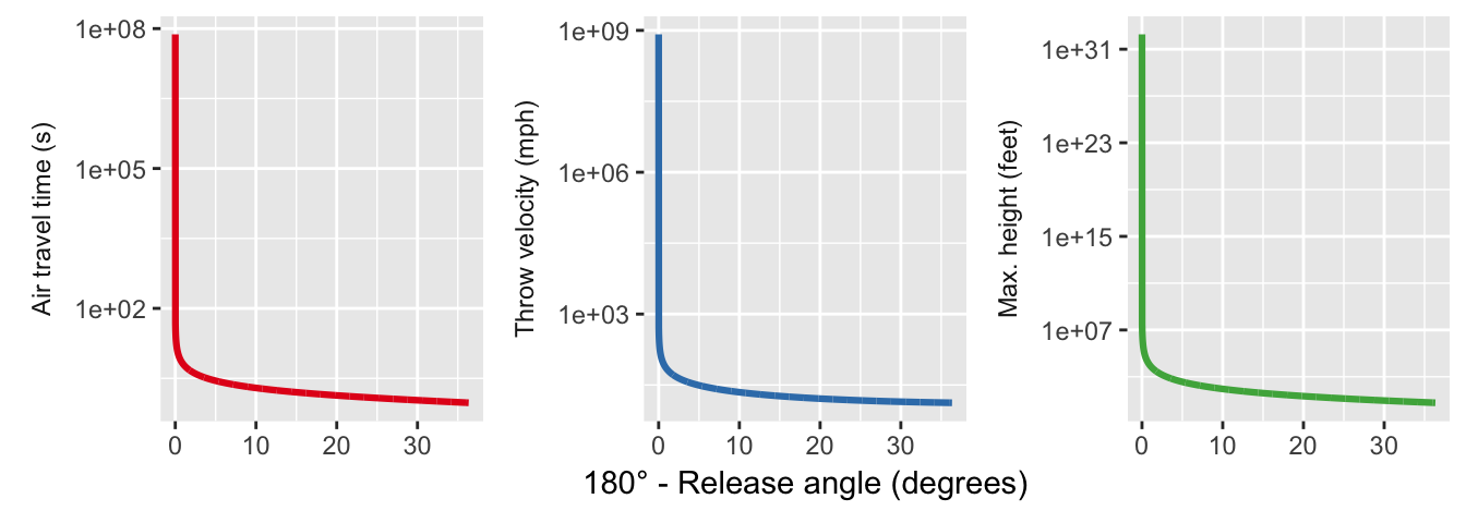
Once again we get crazy behavior with velocity, but now the time and maximum height are both extremely large – these plots are on a logarithmic scale. These solutions basically correspond to throwing a dart upwards and still managing to hit the bullseye. For some of these solutions our constant-$g$ approximation would be in big trouble!

Margin of Error in Release Angle

Finally, what is our margin of error on dart throws? We can check by plotting $\delta y = dy/d\theta \, \delta\theta$ and letting $\delta\theta = 1^\circ$.

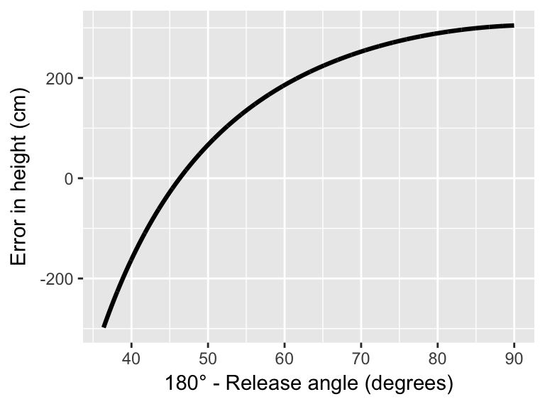
This plot suggests two things:

1. There is an angle near 46 degrees where throws are less affected by errors in angle.
2. The dart can miss by quite a bit for angles far from $46^\circ$: on the order of meters (this seems like quite a lot).

Conclusion

For the set up we considered, it turns out that there is an angle near $\varphi = 46^\circ$ for which the required velocity is a minimum. The dart throw is also most forgiving near that angle. There are also an interesting class of solutions that require fast dart throws, some of which would put the dart into orbit!

This was a fun exercise – I was able to work the problem and do the computation in an evening.